Data Filtering and Selection Techniques

Overview

Introduction

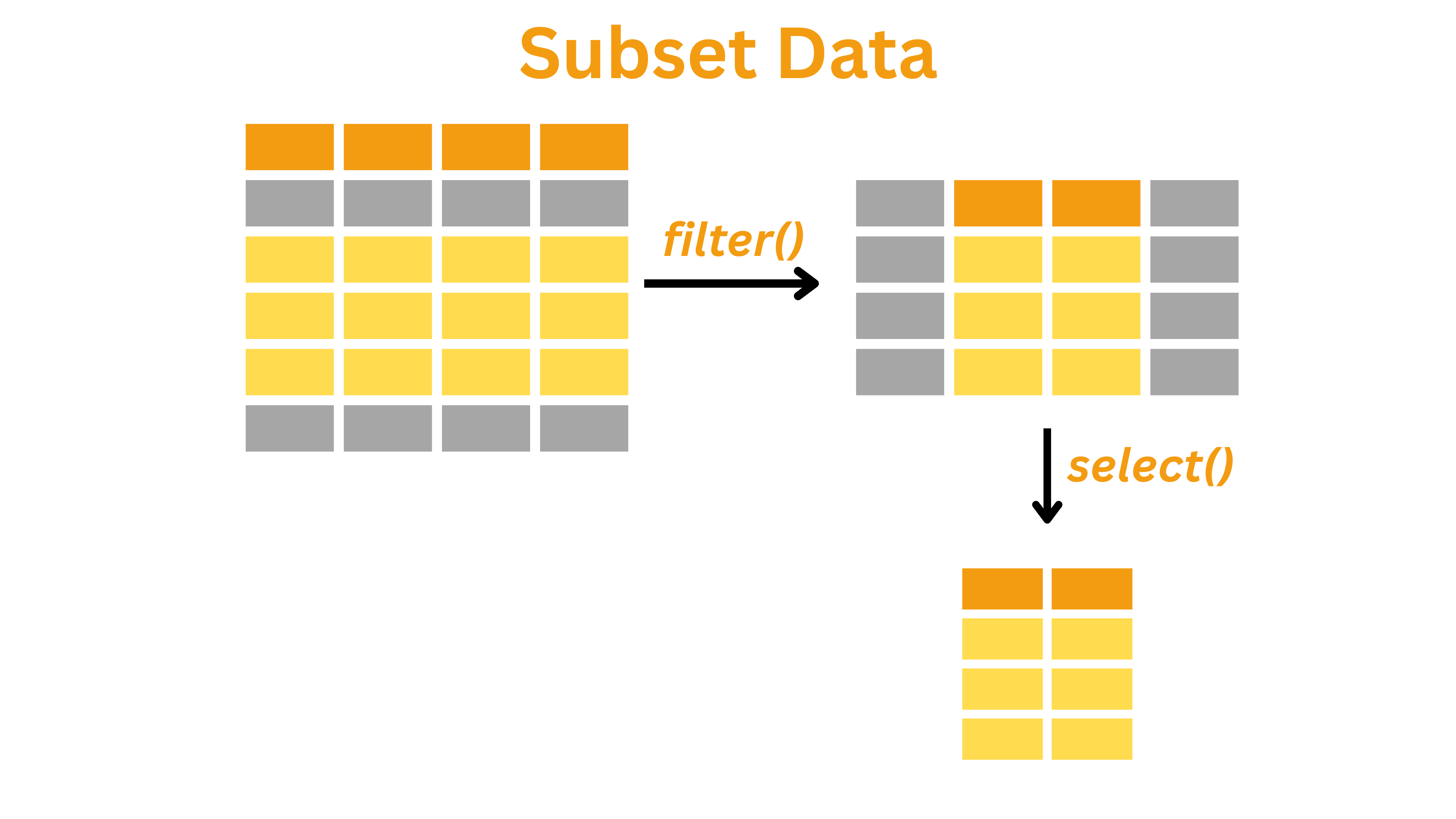
Subsetting data is an essential part of the transform stage in the data science workflow. It involves extracting a portion of the dataset based on specific conditions.

In this short tutorial, we will learn:

1. What subsetting means and why it is crucial
2. How to perform subsetting using conditional operators and the dplyr functions filter() and select()

Why is subsetting a dataset important?

Most real-world datasets are large and complex, with many variables and thousands of records.

Most real-world datasets are large and complex, with many variables and thousands of records. Analyzing all of it at once can introduce noise, slow down computation, and make it harder to detect meaningful patterns. By filtering rows and selecting specific columns, we reduce this complexity, improve clarity, and can more efficiently test hypotheses or build models. Subsetting also plays a key role in ensuring data quality, allowing us to remove irrelevant or problematic entries like missing values, outliers, or categories outside the scope of our analysis.

Filtering rows and selecting specific columns helps us:

• Reduce dataset complexity and improve clarity, making it easier to test hypotheses efficiently
• Remove irrelevant or problematic entries such as missing values, outliers, or unused categories, improving overall data quality

The original dataset is very large—it includes 848 variables and 17,000+ observations.

The dataset we have used in previous sessions originated from the [General Social Survey, Cycle 29 (2015)] (https://odesi.ca/en/details?id=/odesi/doi__10-5683_SP3_RDS0CK.xml), from the Social and Aboriginal Statistics Division at Statistics Canada. This survey tracks how Canadians spend and manage their time, helping us understand patterns tied to well-being and stress. However, the original dataset is very large—it includes over 848 variables and more than 17,000 observations.

For the purposes of this tutorial, we are not interested in every variable. Instead, we are working with a subset of this dataset: 29 variables focused mainly on time durations and key demographic characteristics. This makes the data more manageable and relevant for our exploration of time use and perceptions of time pressure.

Framing the Guiding Question: Who Feels Rushed?

Let’s return to the time usage dataset. In this section, suppose we’re interested in understanding how people who feel rushed spend their time differently from those who don’t. To answer this question, we don’t need every single row or column, as working with the data in its original format would be unnecessarily complex. Instead, we need to “get inside” our data by subsetting: filtering the rows and selecting the columns that matter.

We will explore our dataset through one guiding question:

How do people who feel rushed spend their time differently from those who don’t?

We’ll focus on the relevant rows and columns that answer this question.

Step by Step

0: Setup and Load the Data

Load and Understand the Dataset

First, we need to load the necessary libraries for this session.

library(dplyr)

In our subsequent tasks, the dplyr package will be essential for subsetting operations such as filtering rows and selecting columns. We can either continue using the js_data object from the previous section or load the timeuse_day3_1.Rdata file from the data folder.

js_data_path <- "data/timeuse_day3_1.Rdata"
load(js_data_path)

Now, let’s again examine our dataset structure by displaying the first few rows by using head() function.

js_data |>
  head()

id	ageGrp	sex	maritalStat	province	popCenter	eduLevel	feelRushed	extraTime	durSleep	durMealPrep	durEating	durAlone	durDriving	durWork	durShoolSite	durSchoolOnline	durStudy	mainStudy	mainJobHunting	mainWork	worked12m	workedWeek	enrollStat	dailyTexts	timeSlowDown	timeWorkaholic	timeNotFamFriends	timeWantAlone	province_fact	maritalStat_fact	eduLevel_fact
10000	5	1	5	46	1	3	1	1	510	60	120	770	90	0	0	0	0	NA	1	1	1	2	NA	8	2	2	2	2	MB	Divorced	Trade certificate or diploma
10001	5	1	1	59	1	4	3	4	420	150	0	0	0	0	0	0	0	NA	2	1	1	2	NA	1	2	2	2	2	BC	Married	College, CEGEP, or other non-university certificate or dimploma
10002	4	2	1	47	1	5	1	6	570	0	0	630	30	480	0	0	0	NA	NA	NA	1	1	NA	7	2	1	1	1	SK	Married	University certificate or dimploma below the bachelor’s level
10003	6	2	5	35	1	4	2	4	510	10	45	875	80	20	0	0	0	NA	NA	NA	1	1	NA	1	2	2	2	2	ON	Divorced	College, CEGEP, or other non-university certificate or dimploma
10004	2	1	6	35	1	NA	1	3	525	90	40	815	0	0	0	0	0	NA	NA	NA	2	2	NA	1	2	2	2	2	ON	Single, never married	NA
10005	1	1	6	35	1	1	1	6	435	0	0	430	40	530	0	0	0	NA	NA	NA	1	1	NA	2	2	1	1	2	ON	Single, never married	Less than high school dimploma or its equivalent

As we can see, there are 30 columns in the dataset, which is a lot to work with. For now, we can focus on the following key columns:

• id: Record identification
• ageGrp: Age group of respondent (groups of 10)
• sex: Sex of respondent
• maritalStat: Marital status of the respondent
• province: Province of residence
• popCenter: Population centre indicator
• eduLevel: Educational attainment (highest degree)
• feelRushed: General time use – Feel rushed
• extraTime: General time use – Extra time
• durSleep: Duration – Sleeping, resting, relaxing, sick in bed
• durWork: Duration – Paid work
• timeWorkaholic: Perceptions of time – Workaholic
• timeWantAlone: Perceptions of time – Would like more time alone

These columns provide information on demographics, time usage, and time perceptions. We can use them to explore patterns in work-life balance, education, and social time.

Now that we understand our dataset structure, let’s move on to learning how to filter and manipulate this data effectively using Boolean operators in dplyr.

1: Learning About Filtering

Conditional Filtering with Boolean Operators using dplyr

dplyr is a powerful package that lets us extract and transform data with a clear, readable syntax. In dplyr, we use functions like filter(), select(), and mutate() to work with our data. Boolean operators (==, <, >, <=, >=, and !=) are used within these functions to test conditions, and we can combine conditions with & (and) or | (or).

Let’s start by understanding the basic comparison operators that will help us create filtering conditions.

Comparison Operators

Comparison operators allow us to check conditions within our dataset. These return TRUE or FALSE based on whether the condition is met.

Operator	Meaning	Example	Result
==	Equal to	5 == 5	TRUE
!=	Not equal to	5 != 3	TRUE
<	Less than	3 < 5	TRUE
>	Greater than	5 > 3	TRUE
<=	Less than or equal to	3 <= 3	TRUE
>=	Greater than or equal to	5 >= 3	TRUE

Once we understand these basic comparison operators, we can combine them using logical operators to create more complex filtering conditions.

Logical Operators

Logical operators allow us to filter data based on multiple conditions.

Operator	Meaning	Example	Result
&	Logical AND (Both conditions must be TRUE)	(5 > 3) & (4 < 6)	TRUE
|	Logical OR (At least one condition must be TRUE)	(5 > 3) | (4 > 6)	TRUE
!	Logical NOT (Reverses TRUE/FALSE)	!(5 > 3)	FALSE

Let’s try using these logical operators to filter the rows in the following example.

We want to understand whether feeling rushed might relate to how much time is spent on work, sleep, or alone time. Therefore, the columns of interest are feelRushed, durSleep, durWork, and durAlone. First, let’s explore the values in these columns using dplyr.

Let’s look at the unique values in the feelRushed column to understand what categories exist in our data before we start filtering based on these values.

js_data |> 
  distinct(feelRushed)

## # A tibble: 7 × 1
##   feelRushed
##        <dbl>
## 1          1
## 2          3
## 3          2
## 4          4
## 5          5
## 6          6
## 7         NA

Since our duration columns (durSleep, durWork, and durAlone) are continuous numerical variables rather than categorical, it’s more informative to examine their distributions rather than just their unique values. Looking at the distribution helps us understand which values are common, identify patterns, and spot potential outliers:

js_data |> 
  count(durSleep) |> 
  arrange(desc(n)) |> 
  head(10) 

## # A tibble: 10 × 2
##    durSleep     n
##       <dbl> <int>
##  1      480  1323
##  2      540  1223
##  3      510  1093
##  4      450   854
##  5      600   849
##  6      420   810
##  7      570   784
##  8      630   455
##  9      390   443
## 10      660   358

js_data |> 
  count(durWork) |> 
  arrange(desc(n)) |> 
  head(10)

## # A tibble: 10 × 2
##    durWork     n
##      <dbl> <int>
##  1       0 11243
##  2     480   437
##  3     510   237
##  4     450   231
##  5     540   230
##  6     420   213
##  7     600   140
##  8     495   138
##  9     465   125
## 10     525   113

js_data |> 
  count(durAlone) |> 
  arrange(desc(n)) |> 
  head(10) 

## # A tibble: 10 × 2
##    durAlone     n
##       <dbl> <int>
##  1     1440  1459
##  2        0  1122
##  3       60   244
##  4       30   216
##  5      120   198
##  6      180   179
##  7      150   162
##  8       90   159
##  9     1380   156
## 10      240   154

These commands work together to show the most common time patterns:

• count() tallies each duration value,
• arrange(desc(n)) sorts from highest to lowest frequency,
• head(10) keeps only the top 10 results

This quick overview helps us understand typical time allocation patterns for sleep, work, and being alone.

It appears that all the columns contain numeric values. However, as we look at the data dictionary, we’ll see that only durWork, durSleep and durAlone have numeric values that represent real quantities (minutes of work, sleep or time alone in a day). In contrast, the values in the feelRushed column have a different meaning.

Code	Value
1	daily
2	few Times a Week
3	once a Week
4	once a Month
5	less a Month
6	never

2: Apply Basic Filtering

Filtering Rows with dplyr

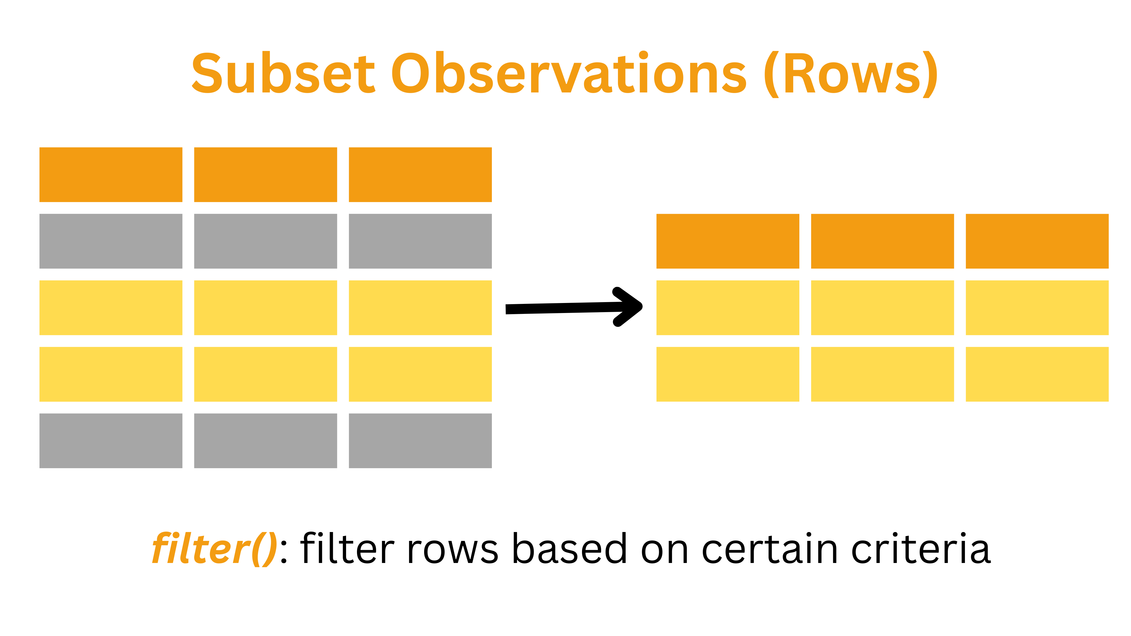
For this analysis, we will consider respondents who report feeling rushed as those whose frequency of feeling this way is at least once a week, and those who feel this way less than once a week as not feeling rushed.

Extracting Respondents Who Do or Do not Feel Rushed Daily

First, let’s extract only the respondents who report feeling rushed daily. Looking at the table, the value corresponding to feeling rushed daily is 1. We can filter for these respondents using filter().

The filter() function in dplyr returns only the rows that meet a specified condition.

We filter any row which has feelRushed equal to 1 by passing the Boolean expression feelRushed == 1 into filter, and then use head() to see what the filtered data look like.

js_data |> 
  filter(feelRushed == 1) |> 
  head()

id	ageGrp	sex	maritalStat	province	popCenter	eduLevel	feelRushed	extraTime	durSleep	durMealPrep	durEating	durAlone	durDriving	durWork	durShoolSite	durSchoolOnline	durStudy	mainStudy	mainJobHunting	mainWork	worked12m	workedWeek	enrollStat	dailyTexts	timeSlowDown	timeWorkaholic	timeNotFamFriends	timeWantAlone	province_fact	maritalStat_fact	eduLevel_fact
10000	5	1	5	46	1	3	1	1	510	60	120	770	90	0	0	0	0	NA	1	1	1	2	NA	8	2	2	2	2	MB	Divorced	Trade certificate or diploma
10002	4	2	1	47	1	5	1	6	570	0	0	630	30	480	0	0	0	NA	NA	NA	1	1	NA	7	2	1	1	1	SK	Married	University certificate or dimploma below the bachelor’s level
10004	2	1	6	35	1	NA	1	3	525	90	40	815	0	0	0	0	0	NA	NA	NA	2	2	NA	1	2	2	2	2	ON	Single, never married	NA
10005	1	1	6	35	1	1	1	6	435	0	0	430	40	530	0	0	0	NA	NA	NA	1	1	NA	2	2	1	1	2	ON	Single, never married	Less than high school dimploma or its equivalent
10011	2	2	6	35	1	3	1	6	630	60	20	235	65	475	0	0	0	NA	NA	NA	1	1	NA	2	1	2	1	2	ON	Single, never married	Trade certificate or diploma
10012	2	2	1	35	2	7	1	2	390	0	50	90	90	480	0	0	0	NA	NA	NA	1	1	NA	2	2	2	1	2	ON	Married	University certificate, diploma, degree above the BA level

Looking at the filtered data, we can confirm that our filter worked correctly—all rows show feelRushed equal to 1 (meaning they feel rushed daily).

Using filter(), we subset the data to keep only those rows where the condition is met. In the above example, the condition feelRushed == 1 creates a logical vector that is TRUE for rows where the value equals 1 (corresponding to “daily”).

Using Comparison and Logical Operators

Not only can we use the == operator to test for equality, but we can also use operators such as <, >, <=, >=, and != to compare values. For example, we might filter rows where a numeric variable exceeds a certain threshold, is below a limit, or is not equal to a specified value. Let’s use an example from the durSleep column.

For instance, if we want to filter rows for the durSleep column to capture any instances with sleep duration less than 600, we can write:

js_data |> 
  filter(durSleep < 600) |>
  head()

id	ageGrp	sex	maritalStat	province	popCenter	eduLevel	feelRushed	extraTime	durSleep	durMealPrep	durEating	durAlone	durDriving	durWork	durShoolSite	durSchoolOnline	durStudy	mainStudy	mainJobHunting	mainWork	worked12m	workedWeek	enrollStat	dailyTexts	timeSlowDown	timeWorkaholic	timeNotFamFriends	timeWantAlone	province_fact	maritalStat_fact	eduLevel_fact
10000	5	1	5	46	1	3	1	1	510	60	120	770	90	0	0	0	0	NA	1	1	1	2	NA	8	2	2	2	2	MB	Divorced	Trade certificate or diploma
10001	5	1	1	59	1	4	3	4	420	150	0	0	0	0	0	0	0	NA	2	1	1	2	NA	1	2	2	2	2	BC	Married	College, CEGEP, or other non-university certificate or dimploma
10002	4	2	1	47	1	5	1	6	570	0	0	630	30	480	0	0	0	NA	NA	NA	1	1	NA	7	2	1	1	1	SK	Married	University certificate or dimploma below the bachelor’s level
10003	6	2	5	35	1	4	2	4	510	10	45	875	80	20	0	0	0	NA	NA	NA	1	1	NA	1	2	2	2	2	ON	Divorced	College, CEGEP, or other non-university certificate or dimploma
10004	2	1	6	35	1	NA	1	3	525	90	40	815	0	0	0	0	0	NA	NA	NA	2	2	NA	1	2	2	2	2	ON	Single, never married	NA
10005	1	1	6	35	1	1	1	6	435	0	0	430	40	530	0	0	0	NA	NA	NA	1	1	NA	2	2	1	1	2	ON	Single, never married	Less than high school dimploma or its equivalent

Alternatively, we can filter rows where durSleep is between 600 and 1000. To do this, we chain two conditions using the & operator:

js_data |> 
  filter(durSleep >= 600 & durSleep <= 1000) |>
  head()

id	ageGrp	sex	maritalStat	province	popCenter	eduLevel	feelRushed	extraTime	durSleep	durMealPrep	durEating	durAlone	durDriving	durWork	durShoolSite	durSchoolOnline	durStudy	mainStudy	mainJobHunting	mainWork	worked12m	workedWeek	enrollStat	dailyTexts	timeSlowDown	timeWorkaholic	timeNotFamFriends	timeWantAlone	province_fact	maritalStat_fact	eduLevel_fact
10006	1	1	6	35	1	1	4	2	635	60	50	650	0	0	0	0	0	NA	2	1	1	2	NA	3	NA	2	2	2	ON	Single, never married	Less than high school dimploma or its equivalent
10011	2	2	6	35	1	3	1	6	630	60	20	235	65	475	0	0	0	NA	NA	NA	1	1	NA	2	1	2	1	2	ON	Single, never married	Trade certificate or diploma
10016	7	1	1	46	2	7	6	6	660	60	0	1440	0	0	0	0	0	NA	2	2	2	2	NA	8	2	2	2	2	MB	Married	University certificate, diploma, degree above the BA level
10021	5	2	1	12	1	6	6	1	660	0	50	640	0	0	0	0	0	NA	2	1	1	2	NA	8	2	2	2	2	NS	Married	Bachelor’s degree
10025	2	1	6	24	1	4	4	6	660	240	60	1440	0	0	0	0	0	NA	NA	NA	1	1	NA	7	2	2	2	2	QC	Single, never married	College, CEGEP, or other non-university certificate or dimploma
10027	1	1	6	13	1	1	2	1	600	0	30	765	0	0	330	0	0	1	1	2	2	2	1	5	1	2	1	2	NB	Single, never married	Less than high school dimploma or its equivalent

In this example:

• The condition durSleep >= 600 checks for rows where sleep duration is at least 600.
• The condition durSleep <= 1000 checks for rows where sleep duration is at most 1000.
• The & operator combines these conditions, ensuring that only rows satisfying both conditions are returned.

Here we’ve used the & operator for “and” conditions, but we can also use the | operator to specify “or” conditions. By using these boolean operators, we can chain multiple conditions together.

3: Apply Complex Filtering

Complex Filtering with dplyr: Filtering Rows for Those Who Feel Rushed

Now, let’s perform a more complex filtering. Suppose we want to capture respondents who feel rushed frequently—that is, those whose feelRushed value is either 1, 2, or 3—and those who do not feel rushed frequently, meaning those whose feelRushed value is either 4, 5, or 6.

There are multiple ways to filter rows that meet one of these conditions.

Using Range Comparison

The first method uses a range comparison with <= to filter the rows.

js_data |> 
  filter(feelRushed <= 3) |>
  head()

id	ageGrp	sex	maritalStat	province	popCenter	eduLevel	feelRushed	extraTime	durSleep	durMealPrep	durEating	durAlone	durDriving	durWork	durShoolSite	durSchoolOnline	durStudy	mainStudy	mainJobHunting	mainWork	worked12m	workedWeek	enrollStat	dailyTexts	timeSlowDown	timeWorkaholic	timeNotFamFriends	timeWantAlone	province_fact	maritalStat_fact	eduLevel_fact
10000	5	1	5	46	1	3	1	1	510	60	120	770	90	0	0	0	0	NA	1	1	1	2	NA	8	2	2	2	2	MB	Divorced	Trade certificate or diploma
10001	5	1	1	59	1	4	3	4	420	150	0	0	0	0	0	0	0	NA	2	1	1	2	NA	1	2	2	2	2	BC	Married	College, CEGEP, or other non-university certificate or dimploma
10002	4	2	1	47	1	5	1	6	570	0	0	630	30	480	0	0	0	NA	NA	NA	1	1	NA	7	2	1	1	1	SK	Married	University certificate or dimploma below the bachelor’s level
10003	6	2	5	35	1	4	2	4	510	10	45	875	80	20	0	0	0	NA	NA	NA	1	1	NA	1	2	2	2	2	ON	Divorced	College, CEGEP, or other non-university certificate or dimploma
10004	2	1	6	35	1	NA	1	3	525	90	40	815	0	0	0	0	0	NA	NA	NA	2	2	NA	1	2	2	2	2	ON	Single, never married	NA
10005	1	1	6	35	1	1	1	6	435	0	0	430	40	530	0	0	0	NA	NA	NA	1	1	NA	2	2	1	1	2	ON	Single, never married	Less than high school dimploma or its equivalent

js_data |> 
  filter(feelRushed > 3 & feelRushed <= 6) |>
  head()

id	ageGrp	sex	maritalStat	province	popCenter	eduLevel	feelRushed	extraTime	durSleep	durMealPrep	durEating	durAlone	durDriving	durWork	durShoolSite	durSchoolOnline	durStudy	mainStudy	mainJobHunting	mainWork	worked12m	workedWeek	enrollStat	dailyTexts	timeSlowDown	timeWorkaholic	timeNotFamFriends	timeWantAlone	province_fact	maritalStat_fact	eduLevel_fact
10006	1	1	6	35	1	1	4	2	635	60	50	650	0	0	0	0	0	NA	2	1	1	2	NA	3	NA	2	2	2	ON	Single, never married	Less than high school dimploma or its equivalent
10007	5	2	3	59	1	4	5	3	440	30	160	1200	60	0	0	0	0	NA	2	2	2	2	NA	8	2	2	1	2	BC	Widowed	College, CEGEP, or other non-university certificate or dimploma
10009	6	1	3	46	1	3	6	2	540	20	120	1060	70	0	0	0	0	NA	2	2	2	2	NA	8	2	2	2	2	MB	Widowed	Trade certificate or diploma
10013	3	1	1	24	1	6	4	6	510	0	20	200	90	0	0	0	0	2	1	2	2	2	2	1	2	1	2	2	QC	Married	Bachelor’s degree
10016	7	1	1	46	2	7	6	6	660	60	0	1440	0	0	0	0	0	NA	2	2	2	2	NA	8	2	2	2	2	MB	Married	University certificate, diploma, degree above the BA level
10021	5	2	1	12	1	6	6	1	660	0	50	640	0	0	0	0	0	NA	2	1	1	2	NA	8	2	2	2	2	NS	Married	Bachelor’s degree

Now let’s calculate how many rows remain after we performed filtering.

all_rows <- js_data |> 
  nrow()
rushed_rows <- js_data |> 
  filter(feelRushed <= 3) |>
  nrow()
not_rushed_rows <- js_data |> 
  filter(feelRushed > 3 & feelRushed <= 6) |>
  nrow()

Let’s print and see the number of rows in each dataframe after filtering.

print(paste("The number of rows in data is:", all_rows))

## [1] "The number of rows in data is: 17390"

print(paste("The number of rows in rushed is:", rushed_rows))

## [1] "The number of rows in rushed is: 12689"

print(paste("The number of rows in not rushed is:", not_rushed_rows))

## [1] "The number of rows in not rushed is: 4639"

• This approach selects rows where feelRushed is less than or equal to 3 (i.e., values 1, 2, or 3) to indicate respondents who feel rushed.
• Rows where feelRushed is greater than or equal to 4 and less than or equal to 6 are considered not rushed.
• We use the & operator to chain the two Boolean operations.
• The nrow() function calculates the number of rows in the data frame.

As we can see, the original data frame has 17,390 rows; after filtering, the rushed data frame contains only 12,689 rows.

Chaining Multiple Conditions

Alternatively, we can use a second method that involves chaining three conditions using the | operator. While this approach is more verbose, it makes the logic very explicit:

js_data |> 
  filter(feelRushed == 1 | feelRushed == 2 | feelRushed == 3) |> 
  head()

id	ageGrp	sex	maritalStat	province	popCenter	eduLevel	feelRushed	extraTime	durSleep	durMealPrep	durEating	durAlone	durDriving	durWork	durShoolSite	durSchoolOnline	durStudy	mainStudy	mainJobHunting	mainWork	worked12m	workedWeek	enrollStat	dailyTexts	timeSlowDown	timeWorkaholic	timeNotFamFriends	timeWantAlone	province_fact	maritalStat_fact	eduLevel_fact
10000	5	1	5	46	1	3	1	1	510	60	120	770	90	0	0	0	0	NA	1	1	1	2	NA	8	2	2	2	2	MB	Divorced	Trade certificate or diploma
10001	5	1	1	59	1	4	3	4	420	150	0	0	0	0	0	0	0	NA	2	1	1	2	NA	1	2	2	2	2	BC	Married	College, CEGEP, or other non-university certificate or dimploma
10002	4	2	1	47	1	5	1	6	570	0	0	630	30	480	0	0	0	NA	NA	NA	1	1	NA	7	2	1	1	1	SK	Married	University certificate or dimploma below the bachelor’s level
10003	6	2	5	35	1	4	2	4	510	10	45	875	80	20	0	0	0	NA	NA	NA	1	1	NA	1	2	2	2	2	ON	Divorced	College, CEGEP, or other non-university certificate or dimploma
10004	2	1	6	35	1	NA	1	3	525	90	40	815	0	0	0	0	0	NA	NA	NA	2	2	NA	1	2	2	2	2	ON	Single, never married	NA
10005	1	1	6	35	1	1	1	6	435	0	0	430	40	530	0	0	0	NA	NA	NA	1	1	NA	2	2	1	1	2	ON	Single, never married	Less than high school dimploma or its equivalent

js_data |> 
  filter(feelRushed == 4 | feelRushed == 5 | feelRushed == 6) |>
  head()

id	ageGrp	sex	maritalStat	province	popCenter	eduLevel	feelRushed	extraTime	durSleep	durMealPrep	durEating	durAlone	durDriving	durWork	durShoolSite	durSchoolOnline	durStudy	mainStudy	mainJobHunting	mainWork	worked12m	workedWeek	enrollStat	dailyTexts	timeSlowDown	timeWorkaholic	timeNotFamFriends	timeWantAlone	province_fact	maritalStat_fact	eduLevel_fact
10006	1	1	6	35	1	1	4	2	635	60	50	650	0	0	0	0	0	NA	2	1	1	2	NA	3	NA	2	2	2	ON	Single, never married	Less than high school dimploma or its equivalent
10007	5	2	3	59	1	4	5	3	440	30	160	1200	60	0	0	0	0	NA	2	2	2	2	NA	8	2	2	1	2	BC	Widowed	College, CEGEP, or other non-university certificate or dimploma
10009	6	1	3	46	1	3	6	2	540	20	120	1060	70	0	0	0	0	NA	2	2	2	2	NA	8	2	2	2	2	MB	Widowed	Trade certificate or diploma
10013	3	1	1	24	1	6	4	6	510	0	20	200	90	0	0	0	0	2	1	2	2	2	2	1	2	1	2	2	QC	Married	Bachelor’s degree
10016	7	1	1	46	2	7	6	6	660	60	0	1440	0	0	0	0	0	NA	2	2	2	2	NA	8	2	2	2	2	MB	Married	University certificate, diploma, degree above the BA level
10021	5	2	1	12	1	6	6	1	660	0	50	640	0	0	0	0	0	NA	2	1	1	2	NA	8	2	2	2	2	NS	Married	Bachelor’s degree

This method very explicitly tests for rows where the feelRushed value is either 1, 2, or 3, or for rows where the value is either 4, 5 or 6.

Again, let’s calculate how many rows remain after we performed filtering.

rushed_rows <- js_data |> 
  filter(feelRushed == 1 | feelRushed == 2 | feelRushed == 3) |>
  nrow()
not_rushed_rows <- js_data |> 
  filter(feelRushed == 4 | feelRushed == 5 | feelRushed == 6) |>
  nrow()

print(paste("The number of rows in rushed is:", rushed_rows))

## [1] "The number of rows in rushed is: 12689"

print(paste("The number of rows in not rushed is:", not_rushed_rows))

## [1] "The number of rows in not rushed is: 4639"

As we can see, looking at the remain rows after filtering, it produces the same output as previously.

There is also a third, more elegant approach using the %in% operator, but we will explore this method in the exercises at the end of this session.

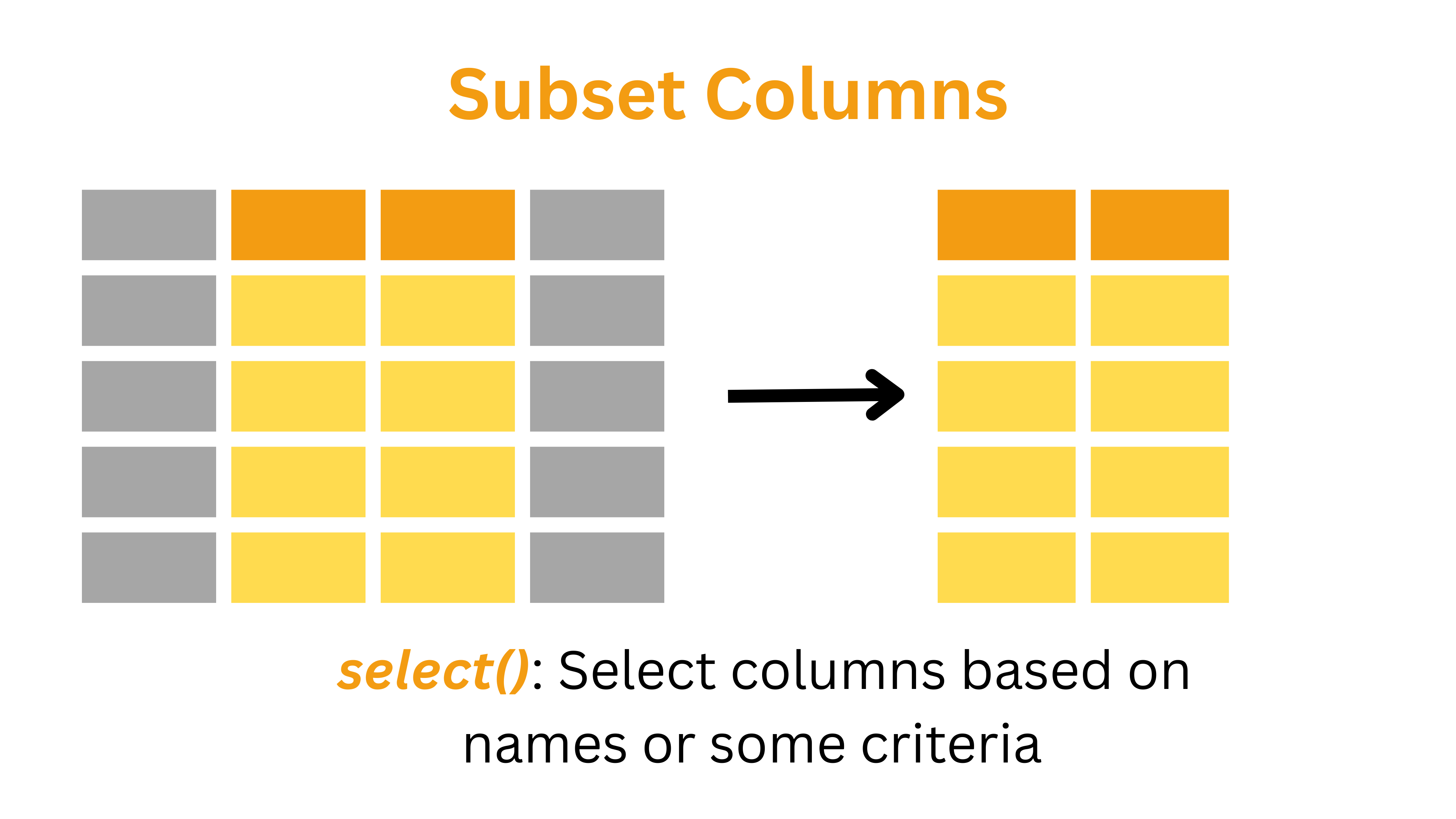
4: Select Relevant Variables

Selecting and Cleaning Time-Related Variables

Next, we’ll focus on the key time allocation columns that are most relevant to our analysis: durWork, durSleep, and durAlone. These variables represent:

• durWork: Time spent on paid work activities
• durSleep: Time spent sleeping, resting, or relaxing
• durAlone: Time spent alone

The select() function in dplyr is used to choose specific columns from a dataset.

We’ll select only these three columns from our rushed and not_rushed datasets using select().

rushed_time <- js_data |> 
  filter(feelRushed <= 3) |>
  select(durWork, durSleep, durAlone) 

not_rushed_time <- js_data |> 
  filter(feelRushed > 3) |> 
  select(durWork, durSleep, durAlone)

In this example, we use the select() function to extract only the relevant columns from the dataset resulting from filtering rows of those who feel rushed (i.e., feelRushed <=3) and those who don’t feel rushed (i.e., feelRushed > 3).

• select(durWork, durSleep, durAlone) tells R to keep only these three columns:
  • durWork: duration of paid work
  • durSleep: duration of sleep and rest
  • durAlone: duration of time spent alone
• The |> (pipe operator) passes the data frames on the left into the select() function.

This step helps reduce the dataset to only the variables we care about for comparing how rushed and not-rushed individuals allocate their time.

In the previous code, we assigned the resulting data frames to the variables not_rushed_time and rushed_time. These variables will be useful when we compare time usage between two groups.

Let’s examine the first few rows of rushed_time and not_rushed_time.

rushed_time |> 
  head()

not_rushed_time |> 
  head()

durWork	durSleep	durAlone
0	510	770
0	420	0
480	570	630
20	510	875
0	525	815
530	435	430

durWork	durSleep	durAlone
0	635	650
0	440	1200
0	540	1060
0	510	200
0	660	1440
0	660	640

As we can see, our data frame resulting from using select() only contain 3 columns: durSleep, durAlone, and durWork

Helper Functions for select()

Suppose we want to pull out every column in js_data whose name refers to “duration”—for example, durWork, durDriving, durSchoolSite, and so on. We could manually list them in select(), but that quickly becomes tedious and error-prone as our data grows.

dplyr provides a family of helper functions for exactly this kind of task. In this case, starts_with("dur") will match every variable whose name begins with “dur”. We can pass that helper directly to select():

js_data |> 
  select(starts_with("dur")) |>
  head()

durSleep	durMealPrep	durEating	durAlone	durDriving	durWork	durShoolSite	durSchoolOnline	durStudy
510	60	120	770	90	0	0	0	0
420	150	0	0	0	0	0	0	0
570	0	0	630	30	480	0	0	0
510	10	45	875	80	20	0	0	0
525	90	40	815	0	0	0	0	0
435	0	0	430	40	530	0	0	0

There are many other helpers, such as ends_with(), contains(), matches(), and more, which let us build clean, flexible code without having to spell out every variable name. We can check the select reference in tidyverse for more information.

5: Compare Time Use

Comparing Time Usage Between Groups

Now that we have our cleaned datasets for both rushed and not rushed groups, we can analyze how these groups differ in their time allocation patterns. We’ll calculate and compare the mean durations for sleep, work, and alone time between the two groups.

Let’s break this down into steps: 1. First, we’ll calculate the mean values for each time-use variable within each group. 2. Then, we’ll compute the differences between these means to understand the magnitude of variation.

We can create a summary table that contains the mean values of durSleep, durAlone, and durWork for each of the rushed_time and not_rushed_time dataframes:

mean_rushed <- rushed_time |> 
  summarise(
    durSleep = mean(durSleep, na.rm = TRUE),
    durAlone = mean(durAlone, na.rm = TRUE),
    durWork = mean(durWork, na.rm = TRUE)
  )

mean_not_rushed <- not_rushed_time |> 
  summarise(
    durSleep = mean(durSleep, na.rm = TRUE),
    durAlone = mean(durAlone, na.rm = TRUE),
    durWork = mean(durWork, na.rm = TRUE)
  )

How it works:

• summarise() collapses each data frame down to a single row.
• Inside, we explicitly name each new column (durSleep, durAlone, durWork) and assign it mean(old_column, na.rm = TRUE).
• na.rm = TRUE makes sure missing values don’t throw off our averages.

However, we can see there’s a little bit of repetition in the code above. We can write much cleaner code to calculate the mean for every column at once.

# Calculate the mean values for each variable using summarise and across
mean_rushed <- rushed_time |> 
  summarise(across(everything(), ~ mean(. , na.rm = TRUE)))

mean_not_rushed <- not_rushed_time |> 
  summarise(across(everything(), ~ mean(. , na.rm = TRUE)))

In this code:

• We use summarise() with across() to calculate means for all columns at once
• The na.rm = TRUE argument ensures we exclude missing values from our calculations

We calculate the difference in means between these two groups.

diff_means <- mean_rushed - mean_not_rushed

The subtraction (mean_rushed - mean_not_rushed) gives a new one‐row tibble showing how much more (or less) time “rushed” individuals spend on each activity compared to “not rushed” individuals.

Now, let’s see what we get up to this point.

## [1] "Mean values for respondents who feel rushed:"

durWork	durSleep	durAlone
203.5197	515.0236	585.7458

## [1] "Mean values for respondents who do not feel rushed:"

durWork	durSleep	durAlone
71.17137	542.4402	773.8862

## [1] "Difference between rushed and not rushed (rushed - not rushed):"

durWork	durSleep	durAlone
132.3483	-27.41654	-188.1403

Positive values in the difference calculation indicate that rushed individuals spend more time on that activity, while negative values indicate they spend less time compared to those who don’t feel rushed.

These results provide interesting insights into how feeling rushed relates to time allocation patterns. For instance, we can observe whether people who feel rushed actually spend more time working or less time sleeping than those who don’t feel rushed, which might help explain their perception of time pressure.

Recode & Save

In the next exercise, we will compare the time pressure felt by respondents based on whether they live in an urban or rural area, as coded in the popCenter column:

js_data |>
  count(popCenter)

## # A tibble: 3 × 2
##   popCenter     n
##       <dbl> <int>
## 1         1 13319
## 2         2  3551
## 3         3   520

According to the data dictionary, these numeric codes mean:

value	label
1	Larger urban population centres (CMA/CA)
2	Rural areas and small population centres (non CMA/CA)
3	Prince Edward Island

We can use dplyr’s mutate() along with if_else() to turn those numbers into descriptive labels:

js_data <- js_data |> mutate(
  popCenter=if_else(popCenter==1,'urban',
                    if_else(popCenter==2,'rural','PEI'))
)

How it works:

• mutate(): adds or modifies columns.
• if_else(condition, true, false): a vectorized, type-safe conditional.
• Here, we nest two if_else() calls so that:
  • popCenter == 1 → “urban”
  • popCenter == 2 → “rural”
  • otherwise (code 3) → “PEI”

Next, we’ll create a new flag called isFeelRushed to mark whether each respondent feels rushed or not. This will be useful for our upcoming data-visualization tutorial:

js_data <- js_data |> mutate(
  isFeelRushed=if_else(feelRushed <= 3,1,0)
)

In this code:

• We assign the result back into js_data so the new column is saved.
• The if_else() function creates a new binary variable:
  • isFeelRushed = 1 if feelRushed is 1, 2, or 3 (i.e. the respondent feels rushed)
  • isFeelRushed = 0 otherwise (i.e. not rushed)

Finally, save the recoded dataset so it’s ready for the next steps:

save(js_data, file = "data/time_use_day3_2.RData")

Exercises: Time for Practice!

Using %in% Operator

In the previous sections, we learned that we can filter respondents who feel rushed or not by either using a range comparison (e.g., feelRushed <= 3) or by chaining multiple conditions with logical operators (e.g., feelRushed == 1 | feelRushed == 2 | feelRushed == 3).

However, there’s also a third, more elegant approach: using the %in% operator. This method is especially helpful when we want to filter a dataset based on multiple specific values of a variable, making our code shorter and easier to read.

Example Scenario

Remember the previous question where we’re analyzing survey data on how frequently people feel rushed. The feelRushed variable includes values from 1 (daily) to 6 (never). We want to group respondents into two categories:

• Rushed: those who feel rushed at least once a week (1, 2, 3)
• Not Rushed: those who feel rushed less often (4, 5, 6)

---

Task Instructions

1. Define the sets of values that represent each group.
2. Use the %in% operator inside filter() to create subsets.
3. Display the first few rows of each subset to verify correctness.
4. Count the number of rows in each group to compare sizes.

---

Steps 1 & 2: Define the sets and use %in% inside filter()

# Define group levels
rushed_levels <- c(1, 2, 3)
not_rushed_levels <- c(4, 5, 6)

# Filter using %in%
js_data |> 
  filter(feelRushed %in% rushed_levels)

js_data |> 
  filter(feelRushed %in% not_rushed_levels)

Step 3a: View the first few rows of rushed_levels

js_data |> 
  filter(feelRushed %in% rushed_levels) |> 
  head()

id	ageGrp	sex	maritalStat	province	popCenter	eduLevel	feelRushed	extraTime	durSleep	durMealPrep	durEating	durAlone	durDriving	durWork	durShoolSite	durSchoolOnline	durStudy	mainStudy	mainJobHunting	mainWork	worked12m	workedWeek	enrollStat	dailyTexts	timeSlowDown	timeWorkaholic	timeNotFamFriends	timeWantAlone	province_fact	maritalStat_fact	eduLevel_fact	isFeelRushed
10000	5	1	5	46	urban	3	1	1	510	60	120	770	90	0	0	0	0	NA	1	1	1	2	NA	8	2	2	2	2	MB	Divorced	Trade certificate or diploma	1
10001	5	1	1	59	urban	4	3	4	420	150	0	0	0	0	0	0	0	NA	2	1	1	2	NA	1	2	2	2	2	BC	Married	College, CEGEP, or other non-university certificate or dimploma	1
10002	4	2	1	47	urban	5	1	6	570	0	0	630	30	480	0	0	0	NA	NA	NA	1	1	NA	7	2	1	1	1	SK	Married	University certificate or dimploma below the bachelor’s level	1
10003	6	2	5	35	urban	4	2	4	510	10	45	875	80	20	0	0	0	NA	NA	NA	1	1	NA	1	2	2	2	2	ON	Divorced	College, CEGEP, or other non-university certificate or dimploma	1
10004	2	1	6	35	urban	NA	1	3	525	90	40	815	0	0	0	0	0	NA	NA	NA	2	2	NA	1	2	2	2	2	ON	Single, never married	NA	1
10005	1	1	6	35	urban	1	1	6	435	0	0	430	40	530	0	0	0	NA	NA	NA	1	1	NA	2	2	1	1	2	ON	Single, never married	Less than high school dimploma or its equivalent	1

Step 3b: View the first few rows of not_rushed_levels

js_data |> 
  filter(feelRushed %in% not_rushed_levels) |> 
  head()

id	ageGrp	sex	maritalStat	province	popCenter	eduLevel	feelRushed	extraTime	durSleep	durMealPrep	durEating	durAlone	durDriving	durWork	durShoolSite	durSchoolOnline	durStudy	mainStudy	mainJobHunting	mainWork	worked12m	workedWeek	enrollStat	dailyTexts	timeSlowDown	timeWorkaholic	timeNotFamFriends	timeWantAlone	province_fact	maritalStat_fact	eduLevel_fact	isFeelRushed
10006	1	1	6	35	urban	1	4	2	635	60	50	650	0	0	0	0	0	NA	2	1	1	2	NA	3	NA	2	2	2	ON	Single, never married	Less than high school dimploma or its equivalent	0
10007	5	2	3	59	urban	4	5	3	440	30	160	1200	60	0	0	0	0	NA	2	2	2	2	NA	8	2	2	1	2	BC	Widowed	College, CEGEP, or other non-university certificate or dimploma	0
10009	6	1	3	46	urban	3	6	2	540	20	120	1060	70	0	0	0	0	NA	2	2	2	2	NA	8	2	2	2	2	MB	Widowed	Trade certificate or diploma	0
10013	3	1	1	24	urban	6	4	6	510	0	20	200	90	0	0	0	0	2	1	2	2	2	2	1	2	1	2	2	QC	Married	Bachelor’s degree	0
10016	7	1	1	46	rural	7	6	6	660	60	0	1440	0	0	0	0	0	NA	2	2	2	2	NA	8	2	2	2	2	MB	Married	University certificate, diploma, degree above the BA level	0
10021	5	2	1	12	urban	6	6	1	660	0	50	640	0	0	0	0	0	NA	2	1	1	2	NA	8	2	2	2	2	NS	Married	Bachelor’s degree	0

Step 4: Count rows

rushed_rows <- js_data |> 
  filter(feelRushed %in% rushed_levels) |> 
  nrow()

not_rushed_rows <- js_data |> 
  filter(feelRushed %in% not_rushed_levels) |> 
  nrow()

print(paste("The number of rows in rushed is:", rushed_rows))

## [1] "The number of rows in rushed is: 12689"

print(paste("The number of rows in not rushed is:", not_rushed_rows))

## [1] "The number of rows in not rushed is: 4639"

Summary

This example shows how the %in% operator simplifies filtering when working with categorical variables. It avoids the need to write multiple == and | conditions, making our code cleaner and easier to read.

Time Pressure Analysis

Let’s use our new filtering and selecting skills to explore how people in urban and rural areas differ in terms of time pressure, based on their reported extra time.

Task Instructions

1. Explore the popCenter and extraTime columns to understand the variable types and possible values.
2. Filter the dataset into two groups: urban and rural.
3. Select the relevant variables: popCenter, extraTime, durWork, and durSleep.
4. Calculate and compare the average extraTime between the two groups.

Step 1: Explore the Data

js_data |> 
  distinct(popCenter)

popCenter
urban
rural
PEI

js_data |> 
  count(extraTime) |> 
  arrange(desc(n)) |> 
  head()

extraTime	n
6	6954
3	2891
2	2662
4	2067
5	1427
1	1313

Step 2: Filter Urban and Rural Populations

To filter the urban population, we use the filter() function to keep only rows where popCenter is equal to "urban". Then, we use head() to display the first few rows of the resulting dataframe:

js_data |> 
  filter(popCenter == 'urban') |>
  head()

id	ageGrp	sex	maritalStat	province	popCenter	eduLevel	feelRushed	extraTime	durSleep	durMealPrep	durEating	durAlone	durDriving	durWork	durShoolSite	durSchoolOnline	durStudy	mainStudy	mainJobHunting	mainWork	worked12m	workedWeek	enrollStat	dailyTexts	timeSlowDown	timeWorkaholic	timeNotFamFriends	timeWantAlone	province_fact	maritalStat_fact	eduLevel_fact	isFeelRushed
10000	5	1	5	46	urban	3	1	1	510	60	120	770	90	0	0	0	0	NA	1	1	1	2	NA	8	2	2	2	2	MB	Divorced	Trade certificate or diploma	1
10001	5	1	1	59	urban	4	3	4	420	150	0	0	0	0	0	0	0	NA	2	1	1	2	NA	1	2	2	2	2	BC	Married	College, CEGEP, or other non-university certificate or dimploma	1
10002	4	2	1	47	urban	5	1	6	570	0	0	630	30	480	0	0	0	NA	NA	NA	1	1	NA	7	2	1	1	1	SK	Married	University certificate or dimploma below the bachelor’s level	1
10003	6	2	5	35	urban	4	2	4	510	10	45	875	80	20	0	0	0	NA	NA	NA	1	1	NA	1	2	2	2	2	ON	Divorced	College, CEGEP, or other non-university certificate or dimploma	1
10004	2	1	6	35	urban	NA	1	3	525	90	40	815	0	0	0	0	0	NA	NA	NA	2	2	NA	1	2	2	2	2	ON	Single, never married	NA	1
10005	1	1	6	35	urban	1	1	6	435	0	0	430	40	530	0	0	0	NA	NA	NA	1	1	NA	2	2	1	1	2	ON	Single, never married	Less than high school dimploma or its equivalent	1

Similarly, we filter the rural population, then preview the first few rows of the resulting dataframe:

js_data |> 
  filter(popCenter == 'rural') |>
  head()

id	ageGrp	sex	maritalStat	province	popCenter	eduLevel	feelRushed	extraTime	durSleep	durMealPrep	durEating	durAlone	durDriving	durWork	durShoolSite	durSchoolOnline	durStudy	mainStudy	mainJobHunting	mainWork	worked12m	workedWeek	enrollStat	dailyTexts	timeSlowDown	timeWorkaholic	timeNotFamFriends	timeWantAlone	province_fact	maritalStat_fact	eduLevel_fact	isFeelRushed
10008	2	2	1	24	rural	6	2	3	525	40	70	30	5	410	0	0	0	NA	NA	NA	1	1	NA	1	2	2	2	2	QC	Married	Bachelor’s degree	1
10012	2	2	1	35	rural	7	1	2	390	0	50	90	90	480	0	0	0	NA	NA	NA	1	1	NA	2	2	2	1	2	ON	Married	University certificate, diploma, degree above the BA level	1
10016	7	1	1	46	rural	7	6	6	660	60	0	1440	0	0	0	0	0	NA	2	2	2	2	NA	8	2	2	2	2	MB	Married	University certificate, diploma, degree above the BA level	0
10018	6	2	1	12	rural	1	3	6	510	15	35	740	330	0	0	0	0	NA	NA	NA	1	1	NA	1	1	1	1	2	NS	Married	Less than high school dimploma or its equivalent	1
10030	6	2	1	10	rural	6	1	6	600	135	60	1005	15	0	0	0	0	NA	2	2	2	2	NA	8	2	1	1	1	NL	Married	Bachelor’s degree	1
10036	3	1	2	24	rural	6	1	6	435	0	45	75	30	720	0	0	0	NA	NA	NA	1	1	NA	1	2	2	1	2	QC	Living common-law	Bachelor’s degree	1

Step 3: Select Relevant Variables

We select the following variables:

• popCenter: to indicate group identity (urban vs. rural)
• extraTime: to measure perceived time availability
• durWork: to examine work duration
• durSleep: to evaluate sleep patterns

We start by selecting the relevant columns from the filtered urban dataframe:

urban_selected <- js_data |> 
  filter(popCenter == 'urban') |> 
  select(popCenter, extraTime, durWork, durSleep)

urban_selected |> 
  head()

popCenter	extraTime	durWork	durSleep
urban	1	0	510
urban	4	0	420
urban	6	480	570
urban	4	20	510
urban	3	0	525
urban	6	530	435

Similarly, we select columns from the filtered rural dataframe:

rural_selected <- js_data |> 
  filter(popCenter == 'rural') |> 
  select(popCenter, extraTime, durWork, durSleep) 

popCenter	extraTime	durWork	durSleep
rural	3	410	525
rural	2	480	390
rural	6	0	660
rural	6	0	510
rural	6	0	600
rural	6	720	435

Step 4: Calculate and Compare Mean Extra Time

To calculate the average amount of extra time reported by urban and rural respondents, we use the summarise() function:

mean_urban <- urban_selected |> 
  summarise(avg_extra_time = mean(extraTime, na.rm = TRUE))
mean_rural <- rural_selected |> 
  summarise(avg_extra_time = mean(extraTime, na.rm = TRUE))

## [1] "Mean extra time for Urban respondents:"

avg_extra_time
4.166139

## [1] "Mean extra time for Rural respondents:"

avg_extra_time
4.255018

It seems that, on average, respondents residing in rural areas have more extraTime. Higher values in extraTime indicate greater availability of free time.

Takeaway

In this session, we learned how to filter rows and select specific columns to create a smaller, cleaner dataset that helps us answer our guiding question more efficiently. Using functions from the dplyr package like filter(), select(), and mutate(), we practiced how to:

• Filter rows based on conditions using comparison and logical operators
  
• Select only the variables we care about using select() and helper functions like starts_with()
  
• Use summarise() and across() to calculate mean values for entire groups
  
• Recode variables like popCenter and create new flags like isFeelRushed with mutate()

These techniques help us zoom in on the parts of the data that matter most and prepare for deeper exploration in the next sessions.

---

This work is licensed under a Creative Commons Attribution-NonCommercial 4.0 International License

Built and rendered courtesy of RMarkdown from RStudio