2 Jupyter Notebooks (.ipynb) Files

Author

Daniel Manrique-Castano

Published

December 8, 2025

2.1 Overview

Jupyter Notebooks are Literate Programming, a paradigm introduced by Donald Knuth (1984), where code and natural language documentation are interwoven to create a “computational narrative.” In data curation, preserving this narrative is as important as preserving the raw data.

Curation Goal

Preserve the computational narrative. Our objective is to assess the structural integrity and documentation quality of notebooks to ensure they remain understandable and potentially reproducible for future researchers.

Preservation Risk

Notebooks are notoriously difficult to re-execute. Studies show that as few as 4% of notebooks produce identical results over time due to non-linear execution, hidden state, and undocumented software environments (Pimentel et al. 2019).

Key Curation Objectives:

Format Obsolescence: Checking nbformat versions to ensure compatibility.
Documentation Quality: Calculating the ratio of Markdown to Code cells. A low ratio indicates poor explainability (Rule et al. 2018).
Dependency Awareness: Scanning imports to identify the software environment required for re-execution.

2.2 Setup

We use jsonlite to parse the notebook structure and tidyverse for data manipulation.

2.2.1 R Packages

If you do not have the required packages, run this command once in your R console:

Code

# install.packages(c("tidyverse", "jsonlite", "rstudioapi", "stringr"))

2.2.2 Load libraries

Code

library(tidyverse)
library(jsonlite)   # To parse .ipynb files
library(rstudioapi) # For directory selection
library(stringr)    # For dependency regex

2.3 Select Target Directory

We select the folder containing the .ipynb files.

Note: If running interactively, a dialog box will appear. Otherwise, it defaults to the target_dir parameter.

Code

# 1. Try to select interactively if in RStudio
if (interactive() && .Platform$OS.type == "windows") { 
  selected_dir <- rstudioapi::selectDirectory(caption = "Select Notebook Directory")
} else {
  selected_dir <- NULL
}

# 2. Logic to determine final directory
if (!is.null(selected_dir)) {
  target_dir <- selected_dir
} else {
  target_dir <- params$target_dir
}

print(paste("Analyzing directory:", target_dir))

[1] "Analyzing directory: data/Inspect_ipynb/"

2.4 Find Jupyter Notebooks

We scan the directory for files ending in .ipynb.

Code

ipynb_files <- list.files(
  path = target_dir,
  pattern = "\\.ipynb$", 
  recursive = TRUE, 
  full.names = TRUE, 
  ignore.case = TRUE
)

print(paste("Found", length(ipynb_files), "Jupyter Notebook files."))

[1] "Found 2 Jupyter Notebook files."

Code

head(ipynb_files)

[1] "data/Inspect_ipynb//Widefield_10x_ROIs_KO_Pdgfrb_TDA.ipynb"
[2] "data/Inspect_ipynb//Widefield_20x_ROIs_Pdgfrb_TDA.ipynb"

2.5 Robust Inventory & Extraction

We perform a “Fail-Safe” extraction. If a notebook is corrupted (invalid JSON), the script flags it as INVALID_JSON instead of crashing.

Code

message("Generating Notebook Report...")

# Regex for imports (Basic Python/R)
# Python: import numpy, from sklearn import ...
# R: library(tidyverse), require(data.table)
import_pattern_py <- "^\\s*(?:import|from)\\s+([a-zA-Z0-9_\\.]+)"
import_pattern_r <- "(?:library|require|p_load)\\s*\\(\\s*[\"']?([a-zA-Z0-9\\.]+)[\"']?\\s*\\)"

report <- purrr::map_dfr(ipynb_files, function(file_path) {
  
  fname <- basename(file_path)
  
  tryCatch({
    # Read the JSON structure
    nb_json <- jsonlite::fromJSON(file_path, flatten = FALSE)
    
    # SAFETY CHECK: Ensure it's a list (JSON object)
    if (!is.list(nb_json)) {
      stop("Parsed content is not a JSON object (is it a list?)")
    }

    # --- Metadata Extraction ---
    # Handle metadata being NULL or not a list
    metadata <- nb_json$metadata
    if (is.null(metadata)) {
        display_name <- "Unknown"
        language <- "Unknown"
    } else if (!is.list(metadata)) {
        display_name <- "Error: Metadata not a list"
        language <- "Unknown"
    } else {
        kernelspec <- metadata$kernelspec
        # Kernelspec check
        if (!is.null(kernelspec) && is.list(kernelspec)) {
             display_name <- if(!is.null(kernelspec$display_name)) kernelspec$display_name else "Unknown"
             language <- if(!is.null(kernelspec$language)) kernelspec$language else "Unknown"
        } else {
             display_name <- "Unknown"
             language <- "Unknown"
        }
    }

    format_version <- paste(nb_json$nbformat, nb_json$nbformat_minor, sep=".")
    
    # --- Cell Analysis ---
    cells <- nb_json$cells
    
    if (is.null(cells) || length(cells) == 0) {
      return(tibble(
        FileName = fname, Language = language, Kernel = display_name, NbFormat = format_version,
        TotalCells = 0, MarkdownCells = 0, CodeCells = 0,
        HasOutputs = FALSE, ErrorOutputs = 0, ExecOrderLinear = TRUE,
        Libraries = "", Status = "Empty"
      ))
    }
    
    # Counts
    num_cells <- nrow(cells)
    markdown_cells <- sum(cells$cell_type == "markdown")
    code_cells_df <- cells[cells$cell_type == "code", ]
    num_code_cells <- nrow(code_cells_df)
    
    # --- Code Cell Deep Dive ---
    has_output <- FALSE
    error_count <- 0
    exec_order_linear <- TRUE
    detected_libs <- character(0)
    
    if (num_code_cells > 0) {
      # 1. Check Outputs
      if (!is.null(code_cells_df$outputs)) {
        has_output <- sum(sapply(code_cells_df$outputs, length) > 0) > 0
        
        # Check for Errors
        all_outputs <- unlist(code_cells_df$outputs, recursive = FALSE)
        if (length(all_outputs) > 0) {
          # Safely extract output_type
          # Ensure x is a list/env before $ access
          output_types <- unlist(lapply(all_outputs, function(x) {
              if (is.list(x)) return(x$output_type) else return(NA)
          }))
          error_count <- sum(output_types == "error", na.rm = TRUE)
        }
      }
      
      # 2. Check Execution Order
      exec_counts <- unlist(code_cells_df$execution_count)
      if (!is.null(exec_counts) && length(exec_counts) > 1) {
        valid_counts <- exec_counts[!is.na(exec_counts)]
        if (length(valid_counts) > 1) {
          exec_order_linear <- !is.unsorted(valid_counts)
        }
      }
      
      # 3. Detect Libraries
      # Unlist all source lines directly to handle line-by-line regex anchors correctly
      # (code_cells_df$source is a list of character vectors)
      all_lines <- unlist(code_cells_df$source)
      
      if (length(all_lines) > 0) {
        if (tolower(language) == "python") {
           matches <- str_match(all_lines, import_pattern_py)
           # str_match returns matrix [full_match, group1]
           detected_libs <- unique(matches[,2])
           detected_libs <- detected_libs[!is.na(detected_libs)]
        } else if (tolower(language) == "r") {
           matches <- str_match(all_lines, import_pattern_r)
           detected_libs <- unique(matches[,2])
           detected_libs <- detected_libs[!is.na(detected_libs)]
        }
      }
    }
    
    tibble(
      FileName = fname,
      Language = language,
      Kernel = display_name,
      NbFormat = format_version,
      TotalCells = num_cells,
      MarkdownCells = markdown_cells,
      CodeCells = num_code_cells,
      doc_ratio = round(MarkdownCells / (CodeCells + 0.001), 2),
      HasOutputs = has_output,
      ErrorOutputs = error_count,
      ExecOrderLinear = exec_order_linear,
      Libraries = paste(detected_libs, collapse = ", "),
      Status = "Success"
    )
    
  }, error = function(e) {
    tibble(
      FileName = fname, Language = "ERROR", Kernel = "", NbFormat = "",
      TotalCells = NA, MarkdownCells = NA, CodeCells = NA,
      HasOutputs = NA, ErrorOutputs = NA, ExecOrderLinear = NA,
      Libraries = "", Status = paste("Failed:", e$message)
    )
  })
})

# Display preview
print("--- Jupyter Notebook Report Preview ---")

[1] "--- Jupyter Notebook Report Preview ---"

Code

print(head(report))

# A tibble: 2 × 13
  FileName Language Kernel NbFormat TotalCells MarkdownCells CodeCells doc_ratio
  <chr>    <chr>    <chr>  <chr>         <int>         <int>     <int>     <dbl>
1 Widefie… python   Pytho… 4.5              51            28        23      1.22
2 Widefie… python   Pytho… 4.5              56            36        20      1.8 
# ℹ 5 more variables: HasOutputs <lgl>, ErrorOutputs <int>,
#   ExecOrderLinear <lgl>, Libraries <chr>, Status <chr>

2.6 Visualization: Documentation Quality

We visualize the ratio of Markdown (Text) to Code. A ratio near 0 implies a script with no explanation. A ratio > 1 implies a well-documented narrative.

Code

ggplot(report, aes(x = reorder(FileName, doc_ratio), y = doc_ratio)) +
  geom_col(aes(fill = doc_ratio > 0.5)) +
  coord_flip() +
  geom_hline(yintercept = 0.5, linetype = "dashed", color = "red") +
  scale_fill_manual(values = c("FALSE" = "#D55E00", "TRUE" = "#009E73"), name = "Well Documented?") +
  labs(
    title = "Notebook Documentation Ratio",
    subtitle = "Ratio of Markdown Cells to Code Cells (Target > 0.5)",
    x = "Notebook",
    y = "Markdown / Code Ratio"
  ) +
  theme_minimal()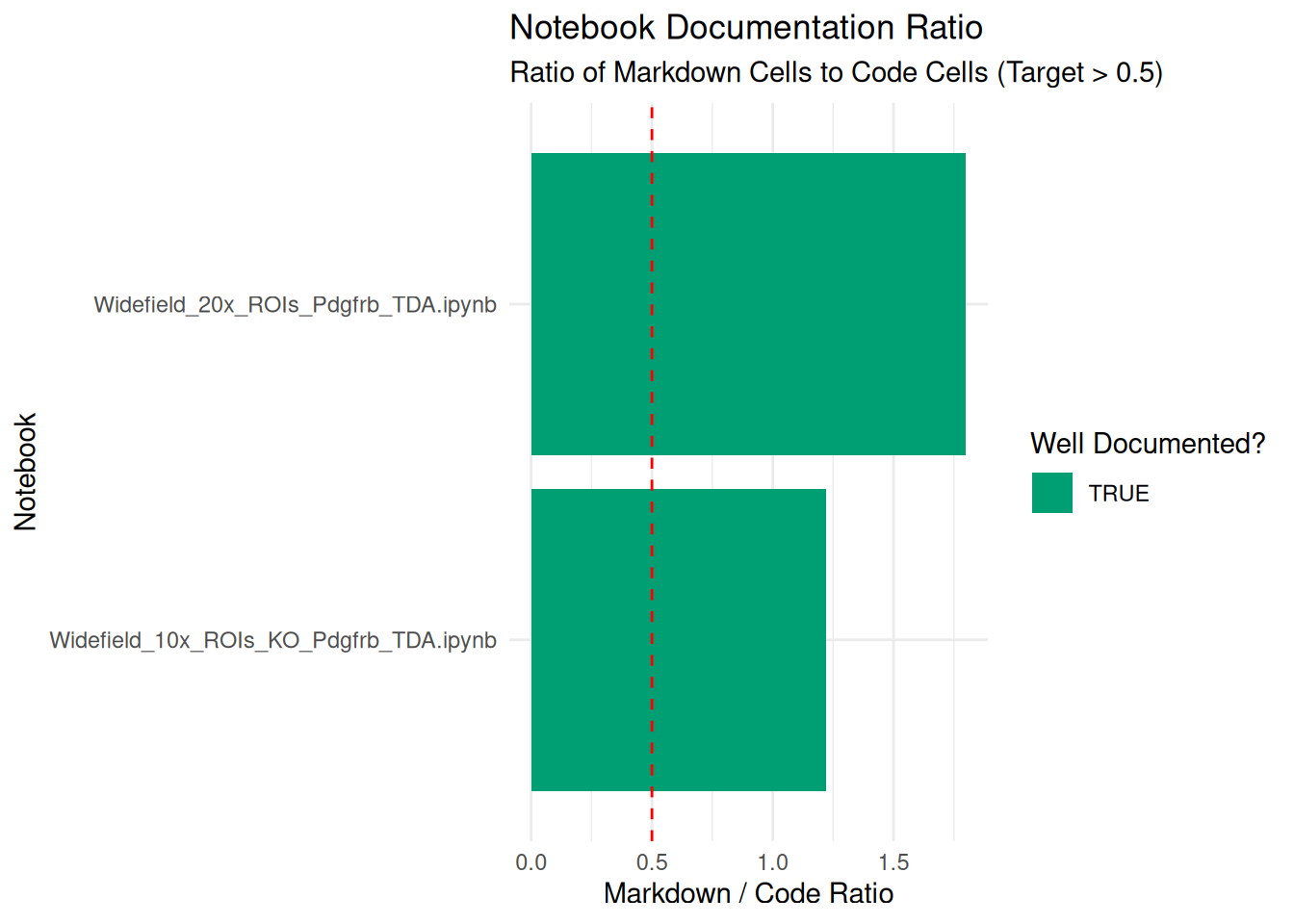

2.7 Save Results

Save the report to a CSV file for review.

Code

output_dir <- "Results/Inspect_ipynb"
dir.create(output_dir, recursive = TRUE, showWarnings = FALSE)

output_file <- file.path(output_dir, paste0("Jupyter_Report_", format(Sys.Date(), "%Y%m%d"), ".csv"))

write.csv(report, output_file, row.names = FALSE)
print(paste("Report saved to:", output_file))

[1] "Report saved to: Results/Inspect_ipynb/Jupyter_Report_20260515.csv"

2.8 Curation Insights

Use the generated CSV to perform these checks:

Residual Outputs (has_outputs): If TRUE, the notebook was saved with graphs, tables, or text logs visible. For archival purposes, it is generally recommended to clear all outputs (using nbstripout or the Jupyter interface). This reduces file size significantly and prevents the accidental leakage of sensitive data (PII) that might be displayed in a table output.
Kernel Consistency: Check for mismatches, such as a notebook using a python2 kernel when the project standard is python3, or a file named Analysis_R.ipynb that actually runs on a python kernel. These inconsistencies often break reproducibility. Ensure the kernel metadata matches the environment provided in requirements.txt or environment.yml.
Format Obsolescence (nbformat): The standard format version is currently 4.x.If you find notebooks with nbformat < 4 (created before ~2015), they may not render correctly in modern JupyterLab. Convert them using nbconvert or open and re-save them in a modern interface.
JSON Validity: Jupyter notebooks are just JSON text files. If the script fails to parse a file, it is likely a “Corrupt Notebook” (invalid JSON structure). Attempt to fix the JSON syntax manually in a text editor, or check if the file was truncated during a previous transfer.

2.9 Additional Tools & Resources

While R parses the metadata efficiently, these specialized tools are essential for managing the notebook lifecycle and reproducibility.

nbstripout: Is a command-line tool that automatically strips output cells from notebooks. It is essential for version control (Git) and preparing “clean” copies for the archive.
Jupytext: This utility converts .ipynb files into paired plain-text scripts (Markdown or Python/R scripts). This allows you to diff changes easily and preserves the code even if the notebook JSON corrupts.
nbconvert: The official tool to convert notebooks into static formats like HTML, PDF, or LaTeX. It is recommended to generate a static HTML or PDF copy of the notebook with outputs executed to ensure the visual results are preserved even if the code stops working in the future.
Binder / Repo2Docker: This utility allows you to build the exact software environment required to run the notebook.

2.10 Using the Non-Interactive R Script

For users who want to run this analysis on a server (HPC), in a batch job, or from the command line, here is the pure R script version.

2.10.1 The `Inspect_ipynb_Script.R` Script

Download the R Script: Inspect_ipynb_Script.R

2.10.2 Example HPC Submission Script (`Inspect_ipynb_submit.sh`)

#!/bin/bash
#SBATCH --job-name=ipynb_inspect
#SBATCH --nodes=1
#SBATCH --ntasks=1
#SBATCH --time=00:15:00
#SBATCH --mem=4G
#SBATCH --output=logs/inspect_ipynb_%j.log

# Load R module (Adjust based on your cluster's module name)
module load R

# Define target directory containing notebooks
TARGET_DIR="/scratch/user/project_data/notebooks"

# Ensure the Results directory exists (optional, script handles it too)
mkdir -p Results/Inspect_ipynb

# Run the R script
echo "Starting Notebook Inspection on $TARGET_DIR"
Rscript Scripts/Inspect_ipynb_Script.R "$TARGET_DIR"

2.11 References

Boettiger, Carl. 2015. “An Introduction to Docker for Reproducible Research.” ACM SIGOPS Operating Systems Review 49 (1): 71–79. https://doi.org/10.1145/2723872.2723882.

Broman, Karl W., and Kara H. Woo. 2018. “Data Organization in Spreadsheets.” The American Statistician 72 (1): 2–10. https://doi.org/10.1080/00031305.2017.1375989.

Brown, Adrian. 2013. Practical Digital Preservation: A How-to Guide for Organizations of Any Size. Facet Publishing.

Cheng, Joe, Barret Schloerke, Bhaskar Karambelkar, and Yihui Xie. 2024. Leaflet: Create Interactive Web Maps with the JavaScript ’Leaflet’ Library. https://CRAN.R-project.org/package=leaflet.

De Wilde, Max, and Ruben Verborgh. 2013. Using OpenRefine: the essential OpenRefine guide that takes you from data analysis and error fixing to linking your dataset to the Web. 1st ed. Community Experience Distilled. Packt Publishing.

Eddelbuettel, Dirk. 2024. Digest: Create Compact Hash Digests of r Objects. https://CRAN.R-project.org/package=digest.

Guide to Social Science Data Preparation and Archiving | ICPSR. n.d. https://www.icpsr.umich.edu/sites/icpsr/manage-data/prepare-deposit/guide.

Hegghammer, Thomas. 2025. daiR: Interface with Google Cloud Document AI API. https://CRAN.R-project.org/package=daiR.

Hester, Jim, Florent Angly, Russ Hyde, et al. 2025. Lintr: A ’Linter’ for r Code. https://CRAN.R-project.org/package=lintr.

Müller, Kirill, Hadley Wickham, David A. James, and Seth Falcon. 2024. RSQLite: ’SQLite’ Interface for r. https://CRAN.R-project.org/package=RSQLite.

O’Brien, Joshua. 2025. Exiftoolr: ExifTool Functionality from r. https://CRAN.R-project.org/package=exiftoolr.

Obe, Regina O., and Leo S. Hsu. 2021. PostGIS in action. Third edition. Manning.

Ooms, Jeroen. 2014. The Jsonlite Package: A Practical and Consistent Mapping Between JSON Data and r Objects. https://arxiv.org/abs/1403.2805.

Ooms, Jeroen. 2025. Magick: Advanced Graphics and Image-Processing in r. https://CRAN.R-project.org/package=magick.

Pebesma, Edzer. 2018. “Simple Features for r: Standardized Support for Spatial Vector Data.” The R Journal 10 (1): 439. https://doi.org/10.32614/rj-2018-009.

Pebesma, Edzer, and Roger Bivand. 2023. Spatial Data Science: With Applications in r. https://doi.org/10.1201/9780429459016.

Pezoa, Felipe, Juan L. Reutter, Fernando Suarez, MartÃn Ugarte, and Domagoj Vrgoč. 2016. “Foundations of JSON Schema.” Proceedings of the 25th International Conference on World Wide Web, April 11, 263–73. https://doi.org/10.1145/2872427.2883029.

Pimentel, Joao Felipe, Leonardo Murta, Vanessa Braganholo, and Juliana Freire. 2019. “A Large-Scale Study about Quality and Reproducibility of Jupyter Notebooks.” 2019 IEEE/ACM 16th International Conference on Mining Software Repositories (MSR), ahead of print, May. https://doi.org/10.1109/msr.2019.00077.

R Core Team. 2024. R: A Language and Environment for Statistical Computing. https://www.R-project.org/.

Rosenthal, David S. H. 2010. “Bit Preservation: A Solved Problem?” International Journal of Digital Curation 5 (1): 134–48. https://doi.org/10.2218/ijdc.v5i1.148.

Rule, Adam, AurÃ©lien Tabard, and James D. Hollan. 2018. “Exploration and Explanation in Computational Notebooks.” Proceedings of the 2018 CHI Conference on Human Factors in Computing Systems, April 19, 1–12. https://doi.org/10.1145/3173574.3173606.

Sachdeva, Mehak. 2024. “Exploratory Spatial Data Analysis.” Geographic Information Science & Technology Body of Knowledge 2024 (1). https://doi.org/10.22224/gistbok/2024.1.28.

Schindelin, Johannes, Ignacio Arganda-Carreras, Erwin Frise, et al. 2012. “Fiji: An Open-Source Platform for Biological-Image Analysis.” Nature Methods 9 (7): 676–82. https://doi.org/10.1038/nmeth.2019.

Stodden, Victoria. 2010. “The Scientific Method in Practice: Reproducibility in the Computational Sciences.” SSRN Electronic Journal, ahead of print. https://doi.org/10.2139/ssrn.1550193.

Tennekes, Martijn. 2018. Tmap: Thematic Maps in r. 84. https://doi.org/10.18637/jss.v084.i06.

Ushey, Kevin, and Hadley Wickham. 2024. Renv: Project Environments. https://CRAN.R-project.org/package=renv.

Warmerdam, Frank. n.d. The Geospatial Data Abstraction Library. Springer Berlin Heidelberg. https://doi.org/10.1007/978-3-540-74831-1_5.

Wickham, Hadley. 2014. “Tidy Data.” Journal of Statistical Software 59 (10). https://doi.org/10.18637/jss.v059.i10.

Wickham, Hadley, Mine Ã‡etinkaya-Rundel, and Grolemund Garret. 2023. R for Data Science. O’Reilly Media, Inc. https://r4ds.hadley.nz/.

Wickham, Hadley, Mara Averick, Jennifer Bryan, et al. 2019. Welcome to the Tidyverse. 4: 1686. https://doi.org/10.21105/joss.01686.

Wickham, Hadley, Evan Miller, and Danny Smith. 2023. Haven: Import and Export ’SPSS’, ’Stata’ and ’SAS’ Files. https://CRAN.R-project.org/package=haven.

Zender, Charles S. 2008. “Analysis of Self-Describing Gridded Geoscience Data with netCDF Operators (NCO).” Environmental Modelling & Software 23 (10-11): 1338–42. https://doi.org/10.1016/j.envsoft.2008.03.004.

2.1 Overview

2.2 Setup

2.2.1 R Packages

2.2.2 Load libraries

2.3 Select Target Directory

2.4 Find Jupyter Notebooks

2.5 Robust Inventory & Extraction

2.6 Visualization: Documentation Quality

2.7 Save Results

2.8 Curation Insights

2.9 Additional Tools & Resources

2.10 Using the Non-Interactive R Script

2.10.1 The Inspect_ipynb_Script.R Script

2.10.2 Example HPC Submission Script (Inspect_ipynb_submit.sh)

2.11 References

2.10.1 The `Inspect_ipynb_Script.R` Script

2.10.2 Example HPC Submission Script (`Inspect_ipynb_submit.sh`)